
1.3.1. numpy array オブジェクト
1.3.1.1. Numpy や numpy array って何
1.3.1.1.1. numpy array オブジェクト
| Python objects: |
|
|---|---|
| Numpy provides: |
|
>>> import numpy as np
>>> a = np.array([0, 1, 2, 3])
>>> a
array([0, 1, 2, 3])
ちなみに
例えば、配列には以下のようなものを入れます:
離散時間ステップでの実験/シミュレーションの値
測定装置に記録された信号、例 音波
画像のピクセル、グレーレベルや色
異なる X-Y-Z 位置で測定された3次元データ、例 MRI スキャン
- ...
どうして便利なの: メモリ効率のよいコンテナが高速な数値操作を提供している。
In [1]: L = range(1000)

In [2]: %timeit [i**2 for i in L]
1000 loops, best of 3: 403 us per loop

In [3]: a = np.arange(1000)

In [4]: %timeit a**2
100000 loops, best of 3: 12.7 us per loop
1.3.1.1.2. Numpy の参考ドキュメント
web では http://docs.scipy.org/
対話的なヘルプ:
In [5]: np.array?
String Form:<built-in function array>
Docstring:
array(object, dtype=None, copy=True, order=None, subok=False, ndmin=0, ...
何か探す:
>>> np.lookfor('create array')
Search results for 'create array'
---------------------------------
numpy.array
    Create an array.
numpy.memmap
    Create a memory-map to an array stored in a *binary* file on disk.
In [6]: np.con*?
np.concatenate
np.conj
np.conjugate
np.convolve
1.3.1.2. 配列の作成
1.3.1.2.1. 配列の手動作成
1次元:
>>> a = np.array([0, 1, 2, 3])
>>> a
array([0, 1, 2, 3])
>>> a.ndim
1
>>> a.shape
(4,)
>>> len(a)
4
2次元、3次元、...:
>>> b = np.array([[0, 1, 2], [3, 4, 5]])    # 2 x 3 array
>>> b
array([[0, 1, 2],
       [3, 4, 5]])
>>> b.ndim
2
>>> b.shape
(2, 3)
>>> len(b)     # returns the size of the first dimension
2

>>> c = np.array([[[1], [2]], [[3], [4]]])
>>> c
array([[[1],
        [2]],

       [[3],
        [4]]])
>>> c.shape
(2, 2, 1)
練習問題: 単純な配列
単純な二次元配列を作りましょう。まず、上の例を再現しましょう。そして次に自分で考えて作ってみましょう: 最初の列に奇数を逆向きに、次の列に偶数を入れてみたものだとどうなりますか。
len()やnumpy.shape()をそれらの配列に対して使ってみましょう。それらの関数はお互いどう関係しているでしょうか。そして配列のndim属性についてはどうでしょうか。
1.3.1.2.2. 配列を作るための関数
ちなみに
実際には、項目一つ一つを入れることは少ない...
1つとばしの値:
>>> a = np.arange(10) # 0 .. n-1  (!)
>>> a
array([0, 1, 2, 3, 4, 5, 6, 7, 8, 9])
>>> b = np.arange(1, 9, 2) # start, end (exclusive), step
>>> b
array([1, 3, 5, 7])
または点の数を指定:
>>> c = np.linspace(0, 1, 6)   # start, end, num-points
>>> c
array([ 0. ,  0.2,  0.4,  0.6,  0.8,  1. ])
>>> d = np.linspace(0, 1, 5, endpoint=False)
>>> d
array([ 0. ,  0.2,  0.4,  0.6,  0.8])
よく使う配列:
>>> a = np.ones((3, 3))  # reminder: (3, 3) is a tuple
>>> a
array([[ 1.,  1.,  1.],
       [ 1.,  1.,  1.],
       [ 1.,  1.,  1.]])
>>> b = np.zeros((2, 2))
>>> b
array([[ 0.,  0.],
       [ 0.,  0.]])
>>> c = np.eye(3)
>>> c
array([[ 1.,  0.,  0.],
       [ 0.,  1.,  0.],
       [ 0.,  0.,  1.]])
>>> d = np.diag(np.array([1, 2, 3, 4]))
>>> d
array([[1, 0, 0, 0],
       [0, 2, 0, 0],
       [0, 0, 3, 0],
       [0, 0, 0, 4]])
np.random: 乱数 (Mersenne Twister 疑似乱数生成器):>>> a = np.random.rand(4) # uniform in [0, 1] >>> a array([ 0.95799151, 0.14222247, 0.08777354, 0.51887998]) >>> b = np.random.randn(4) # Gaussian >>> b array([ 0.37544699, -0.11425369, -0.47616538, 1.79664113]) >>> np.random.seed(1234) # Setting the random seed
練習問題: 関数を使って配列を作る
arange,linspace,ones,zeros,eyeそしてdiagを使って実験します。乱数を使っていろいろな種類の配列を作りましょう。
乱数を使って配列を作る前に乱数の seed を設定しましょう。
np.empty関数を使ってみてみましょう。この関数は何をしますか。どういうときに便利でしょうか。
1.3.1.3. 基本的なデータ型
気づいているかもしれませんが、いくつかの例で配列の要素にドットがついて表示されているものがあります(例 2. vs 2)。これはデータ型の違いによるものです:
>>> a = np.array([1, 2, 3])
>>> a.dtype
dtype('int64')

>>> b = np.array([1., 2., 3.])
>>> b.dtype
dtype('float64')
ちなみに
異なるデータ型を使うことでデータをメモリ上にコンパクトに蓄えることができますが、ほとんどの場合はただ単に浮動小数点数を扱いたいだけです。上の例にあるように NumPy は入力から自動的にデータ型を判別します。
明示的にデータ型を指定したい場合はこうします:
>>> c = np.array([1, 2, 3], dtype=float)
>>> c.dtype
dtype('float64')
デフォルト のデータ型は浮動小数点数です:
>>> a = np.ones((3, 3))
>>> a.dtype
dtype('float64')
別の型もあります:
| Complex: | >>> d = np.array([1+2j, 3+4j, 5+6*1j])
>>> d.dtype
dtype('complex128')
|
|---|---|
| Bool: | >>> e = np.array([True, False, False, True])
>>> e.dtype
dtype('bool')
|
| Strings: | >>> f = np.array(['Bonjour', 'Hello', 'Hallo',])
>>> f.dtype # <--- strings containing max. 7 letters
dtype('S7')
|
| Much more: |
|
1.3.1.4. 基本的な可視化
ここまでで、データ配列に関する第一歩を終えました、それらを可視化してみましょう。
まず IPython を起動しましょう:
$ ipython
または notebook を使ってみるのもいいでしょう:
$ ipython notebook
IPython が起動したら、インタラクティブにプロットできるようにしましょう:
>>> %matplotlib
notebook を使っている場合は、notebook でプロットできるようにします:
>>> %matplotlib inline
notebook 上では inline を使うことは重要です、図は notebook 上で表示され新しいウィンドウでは表示されません。
Matplotlib は 2次元の作画パッケージです。その機能を以下のようにして関数をインポートできます:
>>> import matplotlib.pyplot as plt # the tidy way
次に以下を試してみましょう(%matplotlib を使ってインタラクティブなプロットを有効にしていない場合 show を明示的に使う必要があります)
>>> plt.plot(x, y)       # line plot
>>> plt.show()           # <-- shows the plot (not needed with interactive plots)
``%matplotlib` でインタラクティブなプロットを有効にしている場合は:
>>> plot(x, y) # line plot
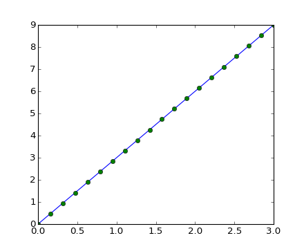
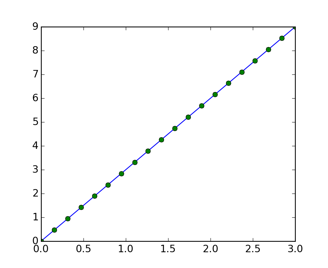
1次元作図:
>>> x = np.linspace(0, 3, 20)
>>> y = np.linspace(0, 9, 20)
>>> plt.plot(x, y)       # line plot
[<matplotlib.lines.Line2D object at ...>]
>>> plt.plot(x, y, 'o')  # dot plot
[<matplotlib.lines.Line2D object at ...>]
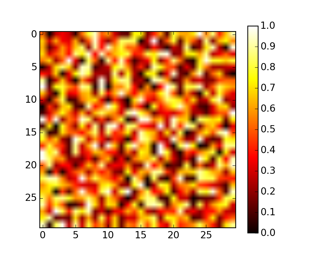
2次元配列 (画像など):
>>> image = np.random.rand(30, 30)
>>> plt.imshow(image, cmap=plt.cm.hot)
>>> plt.colorbar()
<matplotlib.colorbar.Colorbar instance at ...>

参考
matplotlib の章 により詳しい情報があります
練習問題: シンプルな可視化
単純な配列をプロットしてみます: 時間とそれに対する余弦関数や2次元行列を表示してみましょう。
2次元行列については
grayカラーマップを使ってみましょう。
1.3.1.5. インデクスとスライス
配列の要素には Python のシーケンス (例 リスト) と同じようにアクセスと代入ができます:
>>> a = np.arange(10)
>>> a
array([0, 1, 2, 3, 4, 5, 6, 7, 8, 9])
>>> a[0], a[2], a[-1]
(0, 2, 9)
警告
他の Python シーケンスと同様に (そして C/C++ とも同様に) インデクスは 0 から始まります。対照的に Fortran や Matlab ではインデクスは 1 から始まります。
python でよくあるシーケンスの逆順のイディオムもサポートされています:
>>> a[::-1]
array([9, 8, 7, 6, 5, 4, 3, 2, 1, 0])
多次元配列に対しては、インデクスは整数のタプルです:
>>> a = np.diag(np.arange(3))
>>> a
array([[0, 0, 0],
       [0, 1, 0],
       [0, 0, 2]])
>>> a[1, 1]
1
>>> a[2, 1] = 10 # third line, second column
>>> a
array([[ 0,  0,  0],
       [ 0,  1,  0],
       [ 0, 10,  2]])
>>> a[1]
array([0, 1, 0])
注釈
2次元では、最初の次元が 列 に次が 行 に対応します。
多次元では
a,a[0]は指定されていない次元の全ての要素をとると解釈されます。
Slicing: Arrays, like other Python sequences can also be sliced:
>>> a = np.arange(10)
>>> a
array([0, 1, 2, 3, 4, 5, 6, 7, 8, 9])
>>> a[2:9:3] # [start:end:step]
array([2, 5, 8])
最後のインデクスが含まれていないことに注意して下さい!:
>>> a[:4]
array([0, 1, 2, 3])
3つのスライス要素全てが必須というわけではありませ: デフォルトでは start が 0 で end が最後そして step が 1 です:
>>> a[1:3]
array([1, 2])
>>> a[::2]
array([0, 2, 4, 6, 8])
>>> a[3:]
array([3, 4, 5, 6, 7, 8, 9])
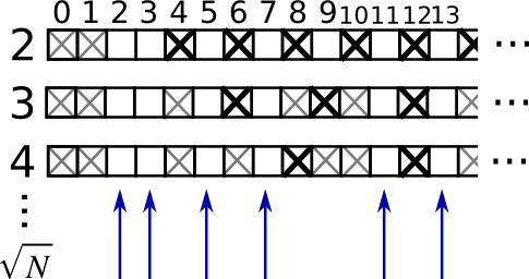
Numpy のインデクスとスライスについて簡単に図示してみると...
代入とスライスを組み合せることもできます:
>>> a = np.arange(10)
>>> a[5:] = 10
>>> a
array([ 0,  1,  2,  3,  4, 10, 10, 10, 10, 10])
>>> b = np.arange(5)
>>> a[5:] = b[::-1]
>>> a
array([0, 1, 2, 3, 4, 4, 3, 2, 1, 0])
練習問題: インデクスとスライス
start,endそしてstepを使ったちょっと毛色の違うスライスも試してみましょう: linspace を使って奇数を逆順に並べ、偶数を順に並べたものを作ってみましょう。上の図で示したスライスを再現してみましょう。以下の表記で配列を作ることもできます:
>>> np.arange(6) + np.arange(0, 51, 10)[:, np.newaxis]
array([[ 0,  1,  2,  3,  4,  5],
       [10, 11, 12, 13, 14, 15],
       [20, 21, 22, 23, 24, 25],
       [30, 31, 32, 33, 34, 35],
       [40, 41, 42, 43, 44, 45],
       [50, 51, 52, 53, 54, 55]])
練習問題: 配列の作成
以下の配列を作成しましょう(正確なデータ型で):
[[1, 1, 1, 1],
 [1, 1, 1, 1],
 [1, 1, 1, 2],
 [1, 6, 1, 1]]

[[0., 0., 0., 0., 0.],
 [2., 0., 0., 0., 0.],
 [0., 3., 0., 0., 0.],
 [0., 0., 4., 0., 0.],
 [0., 0., 0., 5., 0.],
 [0., 0., 0., 0., 6.]]
このコースでのパー: どちらも文3つ
Hint: 配列の各要素にはリストと同じようにアクセスできます 例 a[1] or a[1, 2].
Hint: diag の docstring を見てみましょう。
練習問題: タイル張りの配列作成
np.tile をざっと見て、この関数を使って配列を作ってみましょう:
[[4, 3, 4, 3, 4, 3],
 [2, 1, 2, 1, 2, 1],
 [4, 3, 4, 3, 4, 3],
 [2, 1, 2, 1, 2, 1]]
1.3.1.6. コピーとビュー
スライス操作は元の配列の ビュー を作成します、このビューは配列のデータにアクセスするための方法に過ぎません。そのため元の配列はメモリ上でコピーされることはありません。 np.may_share_memory() を使うことで2つの配列が同じメモリブロックを共有しているか確認することもできます。ただし、この関数はヒューリスティックを使っているため、false positive な結果を返す可能性があります。
ビューを変更すると、元の配列も同様に変更されます:
>>> a = np.arange(10)
>>> a
array([0, 1, 2, 3, 4, 5, 6, 7, 8, 9])
>>> b = a[::2]
>>> b
array([0, 2, 4, 6, 8])
>>> np.may_share_memory(a, b)
True
>>> b[0] = 12
>>> b
array([12,  2,  4,  6,  8])
>>> a   # (!)
array([12,  1,  2,  3,  4,  5,  6,  7,  8,  9])

>>> a = np.arange(10)
>>> c = a[::2].copy()  # force a copy
>>> c[0] = 12
>>> a
array([0, 1, 2, 3, 4, 5, 6, 7, 8, 9])

>>> np.may_share_memory(a, c)
False
この挙動をはじめて見たらおどろくでしょう... しかし、これによって多くのメモリが節約されるのです。
演習例: 素数のふるい
ふるい sieve を使って 0–99 の間の素数を計算しましょう
(100,) のシェイプを持つ、真偽値の配列
is_primeを作成します、最初に True で埋めておきます:
>>> is_prime = np.ones((100,), dtype=bool)
0 と 1 は素数でないので除きます:
>>> is_prime[:2] = 0
2から始まる各整数
jを使ってその積になっているものを除きます:
>>> N_max = int(np.sqrt(len(is_prime)))
>>> for j in range(2, N_max):
...     is_prime[2*j::j] = False
help(np.nonzero)を眺めて、素数を印字しますフォローアップ:
上のコードを
prime_sieve.pyという名前のスクリプトファイルに移す実行して動作しているか確認する
the sieve of Eratosthenes で挙げられている最適化をしてみましょう:
素数でないとわかっている
jについては省く最初に \(j^2\) を除く
1.3.1.7. ファンシーインデクス
ちなみに
Numpy の配列はスライスだけでなく、真偽値や整数配列 (マスク) でもインデクスできます。この方法は ファンシーインデクス と呼ばれています。これは ビューでなくコピー を作ります。
1.3.1.7.1. 真偽値のマスクを利用する
>>> np.random.seed(3)
>>> a = np.random.random_integers(0, 20, 15)
>>> a
array([10,  3,  8,  0, 19, 10, 11,  9, 10,  6,  0, 20, 12,  7, 14])
>>> (a % 3 == 0)
array([False,  True, False,  True, False, False, False,  True, False,
        True,  True, False,  True, False, False], dtype=bool)
>>> mask = (a % 3 == 0)
>>> extract_from_a = a[mask] # or,  a[a%3==0]
>>> extract_from_a           # extract a sub-array with the mask
array([ 3,  0,  9,  6,  0, 12])
マスクによるインデクスは配列内の一部に代入するのに便利に使えます:
>>> a[a % 3 == 0] = -1
>>> a
array([10, -1,  8, -1, 19, 10, 11, -1, 10, -1, -1, 20, -1,  7, 14])
1.3.1.7.2. 整数配列によるインデクス
>>> a = np.arange(0, 100, 10)
>>> a
array([ 0, 10, 20, 30, 40, 50, 60, 70, 80, 90])
インデクス指定は整数配列を使ってもできます、同じインデクスが何回か繰り返されていても使えます:
>>> a[[2, 3, 2, 4, 2]]  # note: [2, 3, 2, 4, 2] is a Python list
array([20, 30, 20, 40, 20])
こんなインデクスを使って新しい値を代入することも可能です:
>>> a[[9, 7]] = -100
>>> a
array([   0,   10,   20,   30,   40,   50,   60, -100,   80, -100])
ちなみに
整数配列によるインデクス指定で新しい配列を作った場合, 新しい配列は整数配列と同じシェイプになります:
>>> a = np.arange(10)
>>> idx = np.array([[3, 4], [9, 7]])
>>> idx.shape
(2, 2)
>>> a[idx]
array([[3, 4],
       [9, 7]])
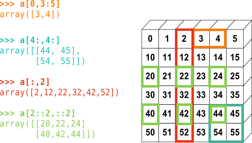
下の画像はいくつかのファンシーインデクスの応用例を示しています
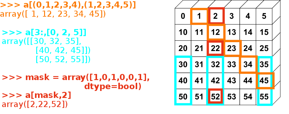
練習問題: ファンシーインデクス
上の図で示されているファンシーインデクスを再現してみましょう。
左にあるファンシーインデクスと右の配列を作成して、配列に値を代入してみましょう、例えば図にある配列の一部を 0 にしてみるなど。