2.5.3. 線形方程式の解法
疎行列の固有値問題ソルバーは
scipy.sparse.linalgにあります- サブモジュール
dsolve: 線形方程式を直接法で分解する方法isolve: 線形方程式を反復法で求解する方法eigen: 疎行列の固有値問題ソルバー
全てのソルバーに以下でアクセスできます:
>>> import scipy.sparse.linalg as spla
>>> spla.__all__
['LinearOperator', 'Tester', 'arpack', 'aslinearoperator', 'bicg',
'bicgstab', 'cg', 'cgs', 'csc_matrix', 'csr_matrix', 'dsolve',
'eigen', 'eigen_symmetric', 'factorized', 'gmres', 'interface',
'isolve', 'iterative', 'lgmres', 'linsolve', 'lobpcg', 'lsqr',
'minres', 'np', 'qmr', 'speigs', 'spilu', 'splu', 'spsolve', 'svd',
'test', 'umfpack', 'use_solver', 'utils', 'warnings']
2.5.3.1. 疎行列の直接法によるソルバー
- デフォルトのソルバー: SuperLU 4.0
SciPy に含まれます
実数及び複素数の方程式系で
単精度及び倍精度の両方
- オプション: umfpack
実数及び複素数の方程式系で
倍精度のみ
パフォーマンスについてはこちらがおすすめ
今では
scikits.umfpackでラッパーが使えますNathaniel Smith による新しい
scikits.suitesparseを確認してみましょう
2.5.3.1.1. 例
モジュール全てをインポートし、ドキュメンテーション文字列をみてみましょう:
>>> from scipy.sparse.linalg import dsolve
>>> help(dsolve)
superlu と umfpack の両方で以下のようにして使うことができます(後者についてはインストールされていれば)
線形方程式の準備:
>>> import numpy as np
>>> from scipy import sparse
>>> mtx = sparse.spdiags([[1, 2, 3, 4, 5], [6, 5, 8, 9, 10]], [0, 1], 5, 5)
>>> mtx.todense()
matrix([[ 1,  5,  0,  0,  0],
        [ 0,  2,  8,  0,  0],
        [ 0,  0,  3,  9,  0],
        [ 0,  0,  0,  4, 10],
        [ 0,  0,  0,  0,  5]])
>>> rhs = np.array([1, 2, 3, 4, 5], dtype=np.float32)
単精度実数として解く:
>>> mtx1 = mtx.astype(np.float32)
>>> x = dsolve.spsolve(mtx1, rhs, use_umfpack=False)
>>> print(x)
[ 106.   -21.     5.5   -1.5    1. ]
>>> print("Error: %s" % (mtx1 * x - rhs))
Error:  [ 0.  0.  0.  0.  0.]
倍精度実数として解く:
>>> mtx2 = mtx.astype(np.float64)
>>> x = dsolve.spsolve(mtx2, rhs, use_umfpack=True)
>>> print(x)
[ 106.   -21.     5.5   -1.5    1. ]
>>> print("Error: %s" % (mtx2 * x - rhs))
Error:  [ 0.  0.  0.  0.  0.]
単精度複素数として解く:
>>> mtx1 = mtx.astype(np.complex64)
>>> x = dsolve.spsolve(mtx1, rhs, use_umfpack=False)
>>> print(x)
[ 106.0+0.j  -21.0+0.j    5.5+0.j   -1.5+0.j    1.0+0.j]
>>> print("Error: %s" % (mtx1 * x - rhs))
Error:  [ 0.+0.j  0.+0.j  0.+0.j  0.+0.j  0.+0.j]
倍精度複素数として解く:
>>> mtx2 = mtx.astype(np.complex128)
>>> x = dsolve.spsolve(mtx2, rhs, use_umfpack=True)
>>> print(x)
[ 106.0+0.j  -21.0+0.j    5.5+0.j   -1.5+0.j    1.0+0.j]
>>> print("Error: %s" % (mtx2 * x - rhs))
Error:  [ 0.+0.j  0.+0.j  0.+0.j  0.+0.j  0.+0.j]
"""
Solve a linear system
=======================

Construct a 1000x1000 lil_matrix and add some values to it, convert it
to CSR format and solve A x = b for x:and solve a linear system with a
direct solver.
"""
import numpy as np
import scipy.sparse as sps
from matplotlib import pyplot as plt
from scipy.sparse.linalg.dsolve import linsolve

rand = np.random.rand

mtx = sps.lil_matrix((1000, 1000), dtype=np.float64)
mtx[0, :100] = rand(100)
mtx[1, 100:200] = mtx[0, :100]
mtx.setdiag(rand(1000))

plt.clf()
plt.spy(mtx, marker='.', markersize=2)
plt.show()

mtx = mtx.tocsr()
rhs = rand(1000)

x = linsolve.spsolve(mtx, rhs)

print('rezidual: %r' % np.linalg.norm(mtx * x - rhs))
2.5.3.2. 反復解法
isolveモジュールは以下のソルバーを含んでいます:bicg(双共役勾配 BIConjugate Gradient)bicgstab(安定化双共役勾配 BIConjugate Gradient STABilized)cg(共益勾配 Conjugate Gradient) - 正定値対称行列のみcgs(自乗共益勾配 Conjugate Gradient Squared)gmres(一般化最小残差 Generalized Minimal RESidual)minres(最小残差 MINimum RESidual)qmr(準最小残差 Quasi-Minimal Residual)
2.5.3.2.1. 共通のパラメーター
必須:
- A: {疎行列、密行列、線形演算子} : {sparse matrix, dense matrix, LinearOperator}
線形方程式の N x N 行列
- b : {配列, 行列} : {array, matrix}
線形方程式の右辺。(N,) または (N,1) のシェイプを持つ。
オプション:
- x0: {配列、行列} : {array, matrix}
解の初期推定。
- tol : 浮動小数点数 : float
終了条件に達する前の相対許容誤差
- maxiter : 整数 : integer
最大反復回数。maxiter 後は指定した誤差に達していなくても反復を終了します。
- M: {疎行列、密行列、線形演算子} : {sparse matrix, dense matrix, LinearOperator}
A の前処理行列。前処理行列は A の逆行列の近似となる必要があります。効果的な前処理は劇的に収束率を改善し、少ない反復で許容誤差に到達することができます。
- callback: 関数 : function
ユーザが与えた関数が各反復後に呼ばれます。callback(xk) として呼ばれ、ここで xk は各反復後の解ベクトルです。
2.5.3.2.2. 線形演算子クラス
from scipy.sparse.linalg.interface import LinearOperator
行列とベクトルの積を実行する共通のインターフェース
便利な抽象化で、疎行列や密行列をソルバーに渡し 行列の形式によらず 解を扱うことを可能にします。
shape と matvec() を持ちます (いくつかのオプションパラメータも加えて)
例:
>>> import numpy as np
>>> from scipy.sparse.linalg import LinearOperator
>>> def mv(v):
...     return np.array([2*v[0], 3*v[1]])
...
>>> A = LinearOperator((2, 2), matvec=mv)
>>> A
<2x2 LinearOperator with unspecified dtype>
>>> A.matvec(np.ones(2))
array([ 2.,  3.])
>>> A * np.ones(2)
array([ 2.,  3.])
2.5.3.2.3. 前処理に関するいくつかの注意
問題に特有で
開発はしばしば困難です
- よくわからない場合は ILU を試してください
solve内で :fun:`spilu()` で利用できます
2.5.3.3. 固有値問題のソルバー
2.5.3.3.1. eigen モジュール
arpack* 大規模な固有値問題を解くために設計された Fortran77 サブルーチンの集まりlobpcg(局所ブロック前処理つき共役勾配法 Locally Optimal Block Preconditioned Conjugate Gradient Method) * が PyAMG との組み合わせでうまく動作します* Nathan Bell による例:""" Compute eigenvectors and eigenvalues using a preconditioned eigensolver ======================================================================== In this example Smoothed Aggregation (SA) is used to precondition the LOBPCG eigensolver on a two-dimensional Poisson problem with Dirichlet boundary conditions. """ import scipy from scipy.sparse.linalg import lobpcg from pyamg import smoothed_aggregation_solver from pyamg.gallery import poisson N = 100 K = 9 A = poisson((N,N), format='csr') # create the AMG hierarchy ml = smoothed_aggregation_solver(A) # initial approximation to the K eigenvectors X = scipy.rand(A.shape[0], K) # preconditioner based on ml M = ml.aspreconditioner() # compute eigenvalues and eigenvectors with LOBPCG W,V = lobpcg(A, X, M=M, tol=1e-8, largest=False) #plot the eigenvectors import pylab pylab.figure(figsize=(9,9)) for i in range(K): pylab.subplot(3, 3, i+1) pylab.title('Eigenvector %d' % i) pylab.pcolor(V[:,i].reshape(N,N)) pylab.axis('equal') pylab.axis('off') pylab.show()
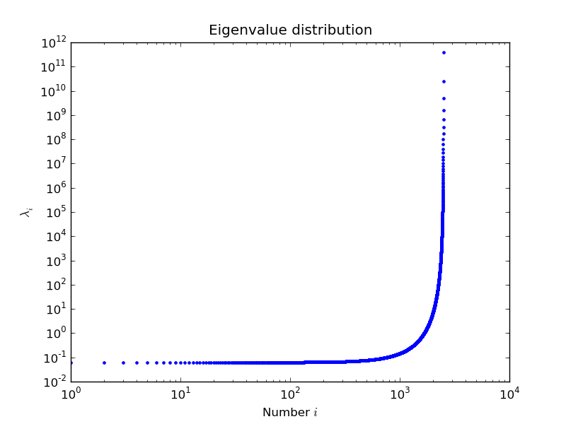
Nils Wagner による例:
出力:
$ python examples/lobpcg_sakurai.py
Results by LOBPCG for n=2500

[ 0.06250083  0.06250028  0.06250007]

Exact eigenvalues

[ 0.06250005  0.0625002   0.06250044]

Elapsed time 7.01