2.6. Numpy と Scipy を利用した画像の操作と処理

著者: Emmanuelle Gouillart, Gaël Varoquaux

この節は、科学技術計算コアモジュールである Numpy や Scipy を利用した画像に対する基本的な操作と処理について扱います。このチュートリアルで扱ういくつかの操作は画像処理以外の多次元配列でも役に経つでしょう。特に scipy.ndimage は n-次元の NumPy 配列を操作する関数を提供します。

参考

より進んだ、画像処理や画像特有のルーチンについては Scikit-image: 画像処理 を参照して下さい、そこでは skimage モジュールについて扱っています。

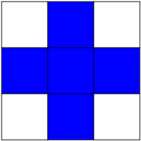
画像 = 2次元の数値配列

(または3次元: CT, MRI, 2次元 + 時間; 4次元, ...)

ここでは 画像 == Numpy 配列 np.array

このチュートリアルで使うツール:

• numpy: 基本的な配列操作

• 画像処理 (n次元画像) 専門の scipy: scipy.ndimage サブモジュールがあります。 ドキュメント を見ましょう:

  >>> from scipy import ndimage
  

画像処理に共通の作業:

• 入出力、画像の表示

• 基本操作: 切り落し、反転、回転、...

• 画像フィルタ: ノイズ除去、シャープにする

• イメージ分割: 異なるオブジェクトに対応するピクセルをラベルづけする

• 分類

• 特徴抽出

• 登録

• ...

2.6.1. 画像ファイルを開く、書き込む

配列をファイルに書き出す:

from scipy import misc
f = misc.face()
misc.imsave('face.png', f) # uses the Image module (PIL)

import matplotlib.pyplot as plt
plt.imshow(f)
plt.show()

画像ファイルから numpy 配列を作る:

>>> from scipy import misc
>>> face = misc.face()
>>> misc.imsave('face.png', face) # First we need to create the PNG file

>>> face = misc.imread('face.png')
>>> type(face)      
<... 'numpy.ndarray'>
>>> face.shape, face.dtype
((768, 1024, 3), dtype('uint8'))

8ビット画像 (0-255) には dtype は unit8 を使います

raw ファイルを開く (カメラや3D画像)

>>> face.tofile('face.raw') # Create raw file
>>> face_from_raw = np.fromfile('face.raw', dtype=np.uint8)
>>> face_from_raw.shape
(2359296,)
>>> face_from_raw.shape = (768, 1024, 3)

画像のシェイプと dtype を知る必要があります (データバイトをどう切り離すか)。

大きいデータに対してはメモリマッピングのために np.memmap 使います:

>>> face_memmap = np.memmap('face.raw', dtype=np.uint8, shape=(768, 1024, 3))

(データはファイルから読み込まれ、メモリに読み込まれません)

画像ファイルのリストを扱ってみます:

>>> for i in range(10):
...     im = np.random.random_integers(0, 255, 10000).reshape((100, 100))
...     misc.imsave('random_%02d.png' % i, im)
>>> from glob import glob
>>> filelist = glob('random*.png')
>>> filelist.sort()

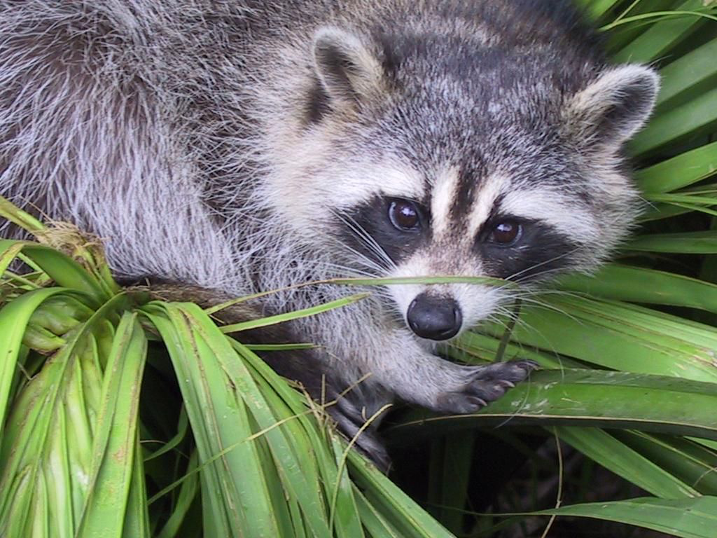
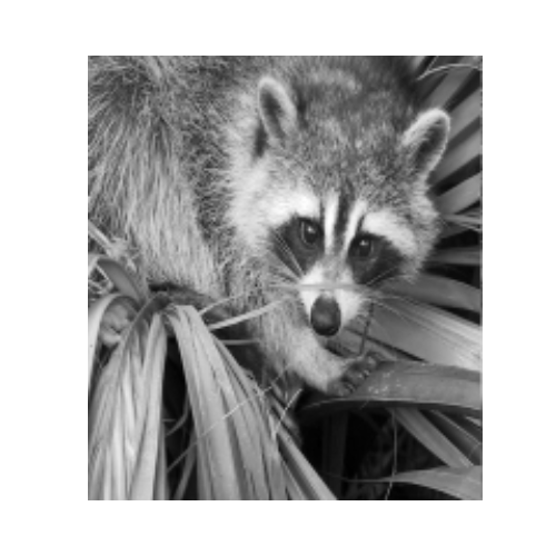
2.6.2. 画像の表示

matplotlib と imshow を利用して画像を matplotlib figure の中に表示します:

>>> f = misc.face(gray=True)  # retrieve a grayscale image
>>> import matplotlib.pyplot as plt
>>> plt.imshow(f, cmap=plt.cm.gray)        
<matplotlib.image.AxesImage object at 0x...>

最大、最小を指定してコントラストを上げます:

>>> plt.imshow(f, cmap=plt.cm.gray, vmin=30, vmax=200)        
<matplotlib.image.AxesImage object at 0x...>
>>> # Remove axes and ticks
>>> plt.axis('off')
(-0.5, 1023.5, 767.5, -0.5)

等高線を描きます:

>>> plt.contour(f, [50, 200])        
<matplotlib.contour.QuadContourSet ...>

[Python source code]

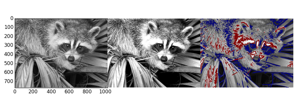
強度の変化をより詳しく調べるために interpolation='nearest' を利用します:

>>> plt.imshow(f[320:340, 510:530], cmap=plt.cm.gray)        
<matplotlib.image.AxesImage object at 0x...>
>>> plt.imshow(f[320:340, 510:530], cmap=plt.cm.gray, interpolation='nearest')        
<matplotlib.image.AxesImage object at 0x...>

[Python source code]

参考

3次元の可視化: Mayavi

Mayavi による 3D プロット を参照。

• 画像の面ウィジェット

• 等高面

• ...

2.6.3. 基本操作

画像は配列です: numpy の仕組み全てを使いましょう。

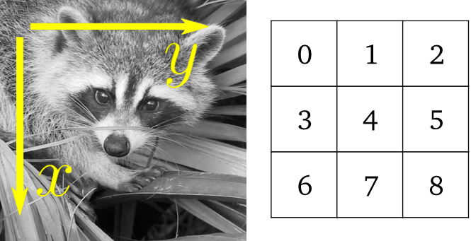
>>> face = misc.face(gray=True)
>>> face[0, 40]
127
>>> # Slicing
>>> face[10:13, 20:23]
array([[141, 153, 145],
       [133, 134, 125],
       [ 96,  92,  94]], dtype=uint8)
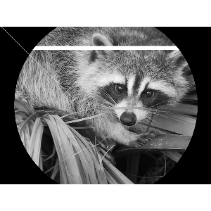
>>> face[100:120] = 255
>>>
>>> lx, ly = face.shape
>>> X, Y = np.ogrid[0:lx, 0:ly]
>>> mask = (X - lx / 2) ** 2 + (Y - ly / 2) ** 2 > lx * ly / 4
>>> # Masks
>>> face[mask] = 0
>>> # Fancy indexing
>>> face[range(400), range(400)] = 255

[Python source code]

2.6.3.1. 統計情報

>>> face = misc.face(gray=True)
>>> face.mean()
113.48026784261067
>>> face.max(), face.min()
(250, 0)

np.histogram

練習問題

• scikit-image のロゴ (http://scikit-image.org/_static/img/logo.png), かコンピュータ上にある画像を配列として開いてみましょう。

• 画像の重要な部分を切り取りましょう、例えばロゴの python が入った丸い部分。

• matplotlib で画像配列を表示します。補間方法を変更し、拡大して差を見てみましょう。

• グレースケールに変換しましょう

• 最大、最小値を変更して画像のコントラストを上げましょう。 任意で: scipy.stats.scoreatpercentile を使って (ドキュメンテーション文字列を読みましょう!) 最も暗いピクセル 5% と最も明るいピクセルの 5% を飽和させてみましょう。

• 配列を異なる2つのファイルフォーマットで保存しましょう (png, jpg, tiff)

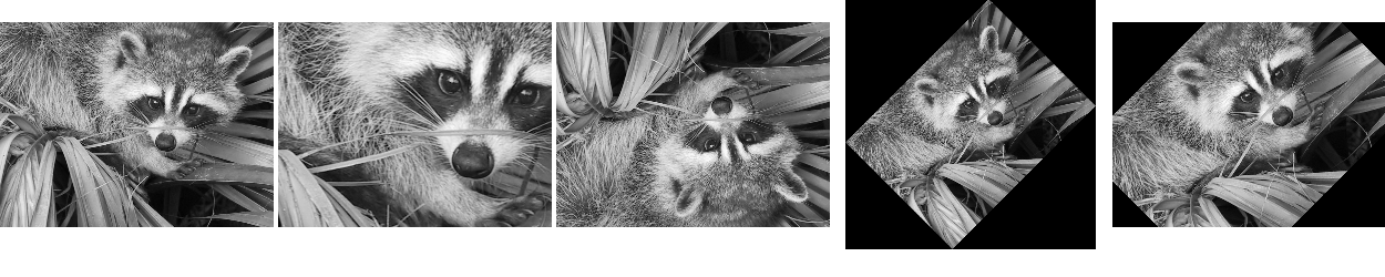
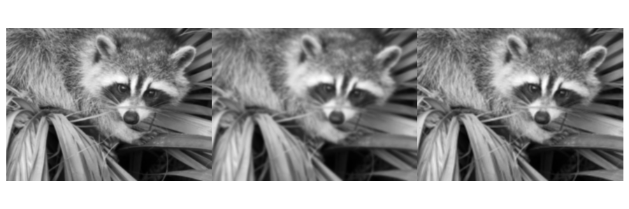
2.6.3.2. 幾何学的変換

>>> face = misc.face(gray=True)
>>> lx, ly = face.shape
>>> # Cropping
>>> crop_face = face[lx / 4: - lx / 4, ly / 4: - ly / 4]
>>> # up <-> down flip
>>> flip_ud_face = np.flipud(face)
>>> # rotation
>>> rotate_face = ndimage.rotate(face, 45)
>>> rotate_face_noreshape = ndimage.rotate(face, 45, reshape=False)

[Python source code]

2.6.4. 画像フィルタ

局所フィルタ: ピクセルの値を、隣接ピクセルの値に応じた関数で置換する。

隣接: 正方形(サイズを選択した)、円形、またはより複雑な 構造要素 。

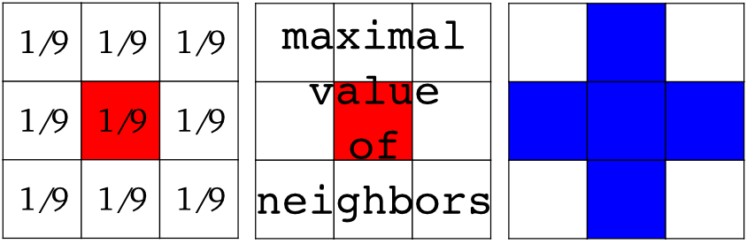
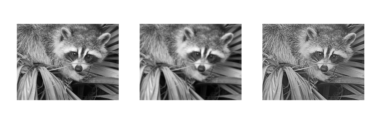
2.6.4.1. ぼかしと平滑化

scipy.ndimage から Gaussian フィルタ

>>> from scipy import misc
>>> face = misc.face(gray=True)
>>> blurred_face = ndimage.gaussian_filter(face, sigma=3)
>>> very_blurred = ndimage.gaussian_filter(face, sigma=5)

一様フィルタ:

>>> local_mean = ndimage.uniform_filter(face, size=11)

[Python source code]

2.6.4.2. シャープにする

ぼかされた画像をシャープに

>>> from scipy import misc
>>> face = misc.face(gray=True).astype(float)
>>> blurred_f = ndimage.gaussian_filter(face, 3)

ラプラシアンの近似を足して、エッジの重みを増やす:

>>> filter_blurred_f = ndimage.gaussian_filter(blurred_f, 1)
>>> alpha = 30
>>> sharpened = blurred_f + alpha * (blurred_f - filter_blurred_f)

[Python source code]

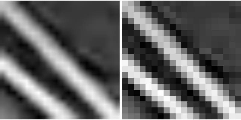
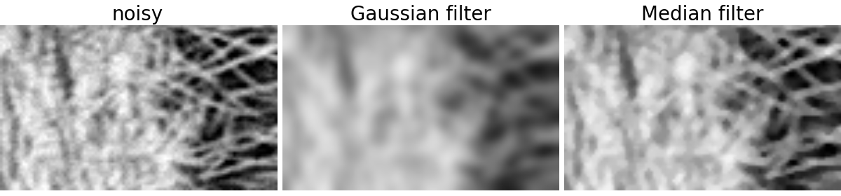
2.6.4.3. ノイズ除去

ノイズの多い顔:

>>> from scipy import misc
>>> f = misc.face(gray=True)
>>> f = f[230:290, 220:320]
>>> noisy = f + 0.4 * f.std() * np.random.random(f.shape)

Gaussian フィルタ はノイズを滑かにします...そしてエッジも同様に:

>>> gauss_denoised = ndimage.gaussian_filter(noisy, 2)

多くの局所的で線形な等方フィルタは画像をぼかします (ndimage.uniform_filter)

メジアンフィルタ はエッジをよく維持してくれます:

>>> med_denoised = ndimage.median_filter(noisy, 3)

[Python source code]

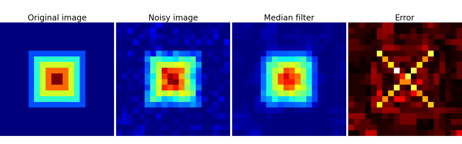
メジアンフィルタ: 直線の境界 (低曲率) に対して良い結果を与えます

>>> im = np.zeros((20, 20))
>>> im[5:-5, 5:-5] = 1
>>> im = ndimage.distance_transform_bf(im)
>>> im_noise = im + 0.2 * np.random.randn(*im.shape)
>>> im_med = ndimage.median_filter(im_noise, 3)

[Python source code]

その他、順序統計量フィルタ: ndimage.maximum_filter, ndimage.percentile_filter

その他の非線形フィルタ: Wiener (scipy.singal.wiener) など。

非局所フィルタ

練習問題: ノイズ除去

• 何かのオブジェクト(円、楕円、正方形、ランダムな形状)でバイナリ画像 (0 か 1 かの) を作成します。

• ノイズを加えます(例えば ノイズを20%)

• 2つの画像ノイズ除去方法を試しましょう: gaussian フィルタやメジアンフィルタ。

• 2つの画像ノイズ除去法のヒストグラムを比較しましょう。どちらのヒストグラムが元の(ノイズのない)画像に近いでしょうか?

参考

より多くのノイズ除去フィルタが skimage.denoising で利用できます、 Scikit-image: 画像処理 のチュートリアルを参照して下さい。

2.6.4.4. 数理形態学

wikipedia を見て、数理形態学の定義を確認しましょう。

画像の中から単純な形状 (構造要素) を検出し、形状が局所的に沿うか沿わないかに応じて画像を変更する

構造要素:

>>> el = ndimage.generate_binary_structure(2, 1)
>>> el
array([[False,  True, False],
       [ True,  True,  True],
       [False,  True, False]], dtype=bool)
>>> el.astype(np.int)
array([[0, 1, 0],
       [1, 1, 1],
       [0, 1, 0]])

Erosion = 最小フィルタ。ピクセルを構造要素を覆うピクセル最小値で置き換える。:

>>> a = np.zeros((7,7), dtype=np.int)
>>> a[1:6, 2:5] = 1
>>> a
array([[0, 0, 0, 0, 0, 0, 0],
       [0, 0, 1, 1, 1, 0, 0],
       [0, 0, 1, 1, 1, 0, 0],
       [0, 0, 1, 1, 1, 0, 0],
       [0, 0, 1, 1, 1, 0, 0],
       [0, 0, 1, 1, 1, 0, 0],
       [0, 0, 0, 0, 0, 0, 0]])
>>> ndimage.binary_erosion(a).astype(a.dtype)
array([[0, 0, 0, 0, 0, 0, 0],
       [0, 0, 0, 0, 0, 0, 0],
       [0, 0, 0, 1, 0, 0, 0],
       [0, 0, 0, 1, 0, 0, 0],
       [0, 0, 0, 1, 0, 0, 0],
       [0, 0, 0, 0, 0, 0, 0],
       [0, 0, 0, 0, 0, 0, 0]])
>>> #Erosion removes objects smaller than the structure
>>> ndimage.binary_erosion(a, structure=np.ones((5,5))).astype(a.dtype)
array([[0, 0, 0, 0, 0, 0, 0],
       [0, 0, 0, 0, 0, 0, 0],
       [0, 0, 0, 0, 0, 0, 0],
       [0, 0, 0, 0, 0, 0, 0],
       [0, 0, 0, 0, 0, 0, 0],
       [0, 0, 0, 0, 0, 0, 0],
       [0, 0, 0, 0, 0, 0, 0]])

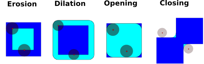
Dilation: 最大フィルタ:

>>> a = np.zeros((5, 5))
>>> a[2, 2] = 1
>>> a
array([[ 0.,  0.,  0.,  0.,  0.],
       [ 0.,  0.,  0.,  0.,  0.],
       [ 0.,  0.,  1.,  0.,  0.],
       [ 0.,  0.,  0.,  0.,  0.],
       [ 0.,  0.,  0.,  0.,  0.]])
>>> ndimage.binary_dilation(a).astype(a.dtype)
array([[ 0.,  0.,  0.,  0.,  0.],
       [ 0.,  0.,  1.,  0.,  0.],
       [ 0.,  1.,  1.,  1.,  0.],
       [ 0.,  0.,  1.,  0.,  0.],
       [ 0.,  0.,  0.,  0.,  0.]])

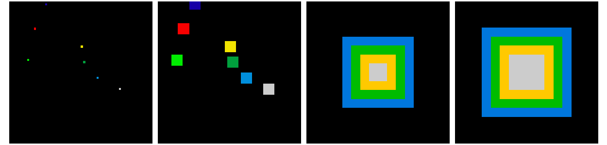
グレー値画像でも動作します:

>>> np.random.seed(2)
>>> im = np.zeros((64, 64))
>>> x, y = (63*np.random.random((2, 8))).astype(np.int)
>>> im[x, y] = np.arange(8)

>>> bigger_points = ndimage.grey_dilation(im, size=(5, 5), structure=np.ones((5, 5)))

>>> square = np.zeros((16, 16))
>>> square[4:-4, 4:-4] = 1
>>> dist = ndimage.distance_transform_bf(square)
>>> dilate_dist = ndimage.grey_dilation(dist, size=(3, 3), \
...         structure=np.ones((3, 3)))

[Python source code]

Opening: erosion + dilation:

>>> a = np.zeros((5,5), dtype=np.int)
>>> a[1:4, 1:4] = 1; a[4, 4] = 1
>>> a
array([[0, 0, 0, 0, 0],
       [0, 1, 1, 1, 0],
       [0, 1, 1, 1, 0],
       [0, 1, 1, 1, 0],
       [0, 0, 0, 0, 1]])
>>> # Opening removes small objects
>>> ndimage.binary_opening(a, structure=np.ones((3,3))).astype(np.int)
array([[0, 0, 0, 0, 0],
       [0, 1, 1, 1, 0],
       [0, 1, 1, 1, 0],
       [0, 1, 1, 1, 0],
       [0, 0, 0, 0, 0]])
>>> # Opening can also smooth corners
>>> ndimage.binary_opening(a).astype(np.int)
array([[0, 0, 0, 0, 0],
       [0, 0, 1, 0, 0],
       [0, 1, 1, 1, 0],
       [0, 0, 1, 0, 0],
       [0, 0, 0, 0, 0]])

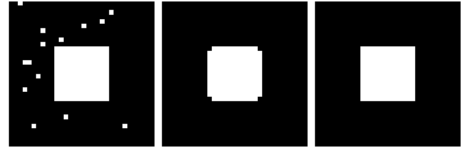
Application: ノイズ除去:

>>> square = np.zeros((32, 32))
>>> square[10:-10, 10:-10] = 1
>>> np.random.seed(2)
>>> x, y = (32*np.random.random((2, 20))).astype(np.int)
>>> square[x, y] = 1

>>> open_square = ndimage.binary_opening(square)

>>> eroded_square = ndimage.binary_erosion(square)
>>> reconstruction = ndimage.binary_propagation(eroded_square, mask=square)

[Python source code]

Closing: dilation + erosion

他の多くの数理形態学演算:: ヒット・ミス演算、tophat など。

2.6.5. 特徴抽出

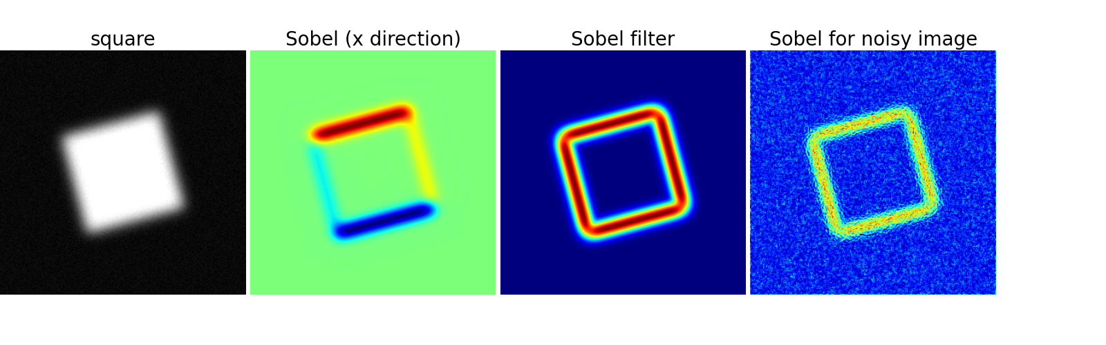
2.6.5.1. エッジ検出

人工データ:

>>> im = np.zeros((256, 256))
>>> im[64:-64, 64:-64] = 1
>>>
>>> im = ndimage.rotate(im, 15, mode='constant')
>>> im = ndimage.gaussian_filter(im, 8)

勾配演算子 (Sobel) を利用して、変化が大きさをとらえる:

>>> sx = ndimage.sobel(im, axis=0, mode='constant')
>>> sy = ndimage.sobel(im, axis=1, mode='constant')
>>> sob = np.hypot(sx, sy)

[Python source code]

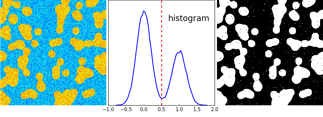
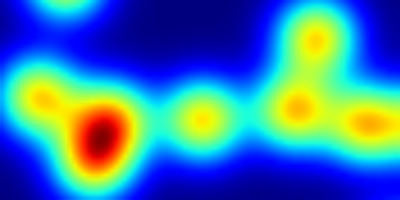
2.6.5.2. 分割

• ヒストグラムを基にした 分割 (空間情報を利用しない)

>>> n = 10
>>> l = 256
>>> im = np.zeros((l, l))
>>> np.random.seed(1)
>>> points = l*np.random.random((2, n**2))
>>> im[(points[0]).astype(np.int), (points[1]).astype(np.int)] = 1
>>> im = ndimage.gaussian_filter(im, sigma=l/(4.*n))

>>> mask = (im > im.mean()).astype(np.float)
>>> mask += 0.1 * im
>>> img = mask + 0.2*np.random.randn(*mask.shape)

>>> hist, bin_edges = np.histogram(img, bins=60)
>>> bin_centers = 0.5*(bin_edges[:-1] + bin_edges[1:])

>>> binary_img = img > 0.5

[Python source code]

数理形態学を利用して、結果をきれいにします:

>>> # Remove small white regions
>>> open_img = ndimage.binary_opening(binary_img)
>>> # Remove small black hole
>>> close_img = ndimage.binary_closing(open_img)

[Python source code]

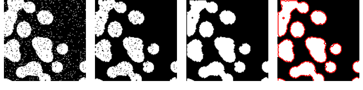
練習問題

再構築演算 (erosion + propagation) で opening/closing よりよい結果が得られることを確認しましょう:

>>> eroded_img = ndimage.binary_erosion(binary_img)
>>> reconstruct_img = ndimage.binary_propagation(eroded_img, mask=binary_img)
>>> tmp = np.logical_not(reconstruct_img)
>>> eroded_tmp = ndimage.binary_erosion(tmp)
>>> reconstruct_final = np.logical_not(ndimage.binary_propagation(eroded_tmp, mask=tmp))
>>> np.abs(mask - close_img).mean() 
0.00727836...
>>> np.abs(mask - reconstruct_final).mean() 
0.00059502...

練習問題

最初のノイズ除去ステップ (例えばメジアンフィルタ) がヒストグラムをどう変化するか確認し、ヒストグラムに基づく分割がより正確になることを確認しましょう。

参考

より進んだ分割アルゴリズムが scikit-image にあります Scikit-image: 画像処理 を参照して下さい。

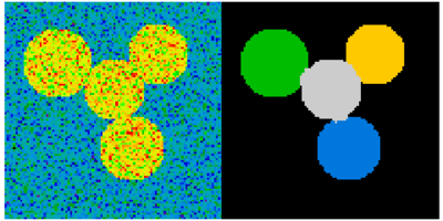
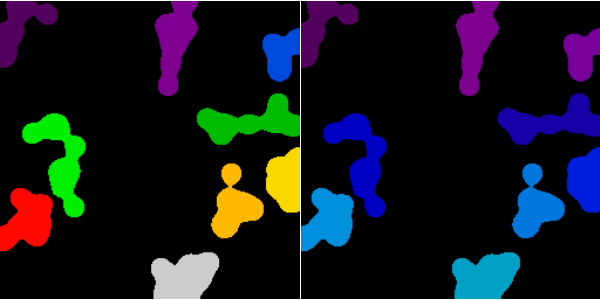
参考

他の科学技術計算パッケージも画像処理に便利なアルゴリズムを提供しています。例えばくっついたオブジェクトを分割するために scikit-learn のスペクトラルクラスタリングを利用します。

>>> from sklearn.feature_extraction import image
>>> from sklearn.cluster import spectral_clustering

>>> l = 100
>>> x, y = np.indices((l, l))

>>> center1 = (28, 24)
>>> center2 = (40, 50)
>>> center3 = (67, 58)
>>> center4 = (24, 70)
>>> radius1, radius2, radius3, radius4 = 16, 14, 15, 14

>>> circle1 = (x - center1[0])**2 + (y - center1[1])**2 < radius1**2
>>> circle2 = (x - center2[0])**2 + (y - center2[1])**2 < radius2**2
>>> circle3 = (x - center3[0])**2 + (y - center3[1])**2 < radius3**2
>>> circle4 = (x - center4[0])**2 + (y - center4[1])**2 < radius4**2

>>> # 4 circles
>>> img = circle1 + circle2 + circle3 + circle4
>>> mask = img.astype(bool)
>>> img = img.astype(float)

>>> img += 1 + 0.2*np.random.randn(*img.shape)
>>> # Convert the image into a graph with the value of the gradient on
>>> # the edges.
>>> graph = image.img_to_graph(img, mask=mask)

>>> # Take a decreasing function of the gradient: we take it weakly
>>> # dependant from the gradient the segmentation is close to a voronoi
>>> graph.data = np.exp(-graph.data/graph.data.std())

>>> labels = spectral_clustering(graph, n_clusters=4, eigen_solver='arpack')
>>> label_im = -np.ones(mask.shape)
>>> label_im[mask] = labels

2.6.6. オブジェクトの性質を計測する: ndimage.measurements

人工データ:

>>> n = 10
>>> l = 256
>>> im = np.zeros((l, l))
>>> points = l*np.random.random((2, n**2))
>>> im[(points[0]).astype(np.int), (points[1]).astype(np.int)] = 1
>>> im = ndimage.gaussian_filter(im, sigma=l/(4.*n))
>>> mask = im > im.mean()

• つながった要素の解析

つながっている要素をラベルづけする: ndimage.label:

>>> label_im, nb_labels = ndimage.label(mask)
>>> nb_labels # how many regions?
16
>>> plt.imshow(label_im)        
<matplotlib.image.AxesImage object at 0x...>

[Python source code]

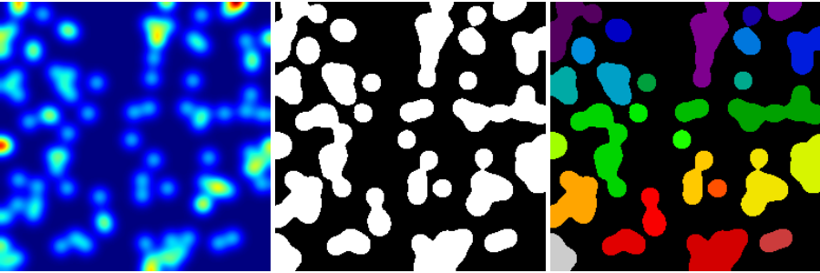
各領域のサイズ、平均値、などを計算する:

>>> sizes = ndimage.sum(mask, label_im, range(nb_labels + 1))
>>> mean_vals = ndimage.sum(im, label_im, range(1, nb_labels + 1))

つながっている要素の内小さいものを消す:

>>> mask_size = sizes < 1000
>>> remove_pixel = mask_size[label_im]
>>> remove_pixel.shape
(256, 256)
>>> label_im[remove_pixel] = 0
>>> plt.imshow(label_im)        
<matplotlib.image.AxesImage object at 0x...>

ラベルを np.searchsoted で再代入します:

>>> labels = np.unique(label_im)
>>> label_im = np.searchsorted(labels, label_im)

[Python source code]

興味あるオブジェクトの領域を見つける:

>>> slice_x, slice_y = ndimage.find_objects(label_im==4)[0]
>>> roi = im[slice_x, slice_y]
>>> plt.imshow(roi)     
<matplotlib.image.AxesImage object at 0x...>

[Python source code]

他の空間的測定:: ndimage.center_of_mass, ndimage.maximum_position など

分割という限られた応用範囲を越えて利用できます。

例: ブロック平均:

>>> from scipy import misc
>>> f = misc.face(gray=True)
>>> sx, sy = f.shape
>>> X, Y = np.ogrid[0:sx, 0:sy]
>>> regions = (sy//6) * (X//4) + (Y//6)  # note that we use broadcasting
>>> block_mean = ndimage.mean(f, labels=regions, index=np.arange(1,
...     regions.max() +1))
>>> block_mean.shape = (sx // 4, sy // 6)

[Python source code]

領域が規則正しいブロックの場合には、ストライドの工夫 (例: ストライドで次元を偽装する) でより効率的にできます。

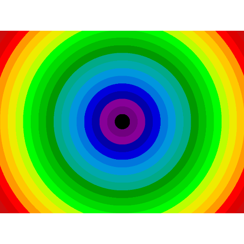
不規則に並ぶブロック: 放射形の平均:

>>> sx, sy = f.shape
>>> X, Y = np.ogrid[0:sx, 0:sy]
>>> r = np.hypot(X - sx/2, Y - sy/2)
>>> rbin = (20* r/r.max()).astype(np.int)
>>> radial_mean = ndimage.mean(f, labels=rbin, index=np.arange(1, rbin.max() +1))

[Python source code]

• 他の計測

相関関数、Fourier/ウェーブレットスペクトル、など。

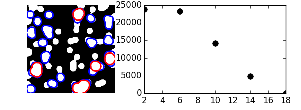
数理形態学の例: granulometry

>>> def disk_structure(n):
...     struct = np.zeros((2 * n + 1, 2 * n + 1))
...     x, y = np.indices((2 * n + 1, 2 * n + 1))
...     mask = (x - n)**2 + (y - n)**2 <= n**2
...     struct[mask] = 1
...     return struct.astype(np.bool)
...
>>>
>>> def granulometry(data, sizes=None):
...     s = max(data.shape)
...     if sizes == None:
...         sizes = range(1, s/2, 2)
...     granulo = [ndimage.binary_opening(data, \
...         structure=disk_structure(n)).sum() for n in sizes]
...     return granulo
...
>>>
>>> np.random.seed(1)
>>> n = 10
>>> l = 256
>>> im = np.zeros((l, l))
>>> points = l*np.random.random((2, n**2))
>>> im[(points[0]).astype(np.int), (points[1]).astype(np.int)] = 1
>>> im = ndimage.gaussian_filter(im, sigma=l/(4.*n))
>>>
>>> mask = im > im.mean()
>>>
>>> granulo = granulometry(mask, sizes=np.arange(2, 19, 4))

[Python source code]

参考

画像処理についてより詳しく:

• Scikit-image の章

• 他にも、より強力で備わったモジュール: OpenCV (Python bindings), CellProfiler, ITK Python bindings つき