
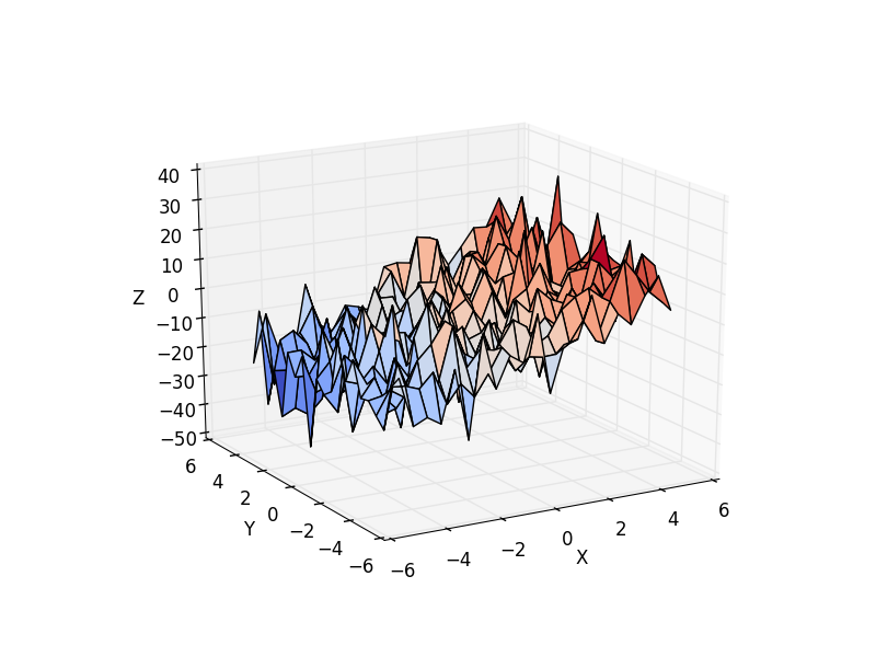
3.1.6.1.1.6. Multiple Regression
Calculate using ‘statsmodels’ just the best fit, or all the corresponding statistical parameters.
Also shows how to make 3d plots.
スクリプトの出力:
  OLS Regression Results
==============================================================================
Dep. Variable:                      z   R-squared:                       0.594
Model:                            OLS   Adj. R-squared:                  0.592
Method:                 Least Squares   F-statistic:                     320.4
Date:                Wed, 03 Feb 2016   Prob (F-statistic):           1.89e-86
Time:                        12:45:22   Log-Likelihood:                -1537.7
No. Observations:                 441   AIC:                             3081.
Df Residuals:                     438   BIC:                             3094.
Df Model:                           2
==============================================================================
                 coef    std err          t      P>|t|      [95.0% Conf. Int.]
------------------------------------------------------------------------------
Intercept     -4.5052      0.378    -11.924      0.000        -5.248    -3.763
x              3.1173      0.125     24.979      0.000         2.872     3.363
y             -0.5109      0.125     -4.094      0.000        -0.756    -0.266
==============================================================================
Omnibus:                        0.260   Durbin-Watson:                   2.057
Prob(Omnibus):                  0.878   Jarque-Bera (JB):                0.204
Skew:                          -0.052   Prob(JB):                        0.903
Kurtosis:                       3.015   Cond. No.                         3.03
==============================================================================

Retrieving manually the parameter estimates:
[-4.50523303  3.11734237 -0.51091248]

ANOVA results
           df        sum_sq       mean_sq           F        PR(>F)
x           1  39284.301219  39284.301219  623.962799  2.888238e-86
y           1   1055.220089   1055.220089   16.760336  5.050899e-05
Residual  438  27576.201607     62.959364         NaN           NaN
Python ソースコード: plot_regression_3d.py
# Original author: Thomas Haslwanter

import numpy as np
import matplotlib.pyplot as plt
import pandas

# For 3d plots. This import is necessary to have 3D plotting below
from mpl_toolkits.mplot3d import Axes3D

# For statistics. Requires statsmodels 5.0 or more
from statsmodels.formula.api import ols
# Analysis of Variance (ANOVA) on linear models
from statsmodels.stats.anova import anova_lm

##############################################################################
# Generate and show the data
x = np.linspace(-5, 5, 21)
# We generate a 2D grid
X, Y = np.meshgrid(x, x)

# To get reproducable values, provide a seed value
np.random.seed(1)

# Z is the elevation of this 2D grid
Z = -5 + 3*X - 0.5*Y + 8 * np.random.normal(size=X.shape)

# Plot the data
fig = plt.figure()
ax = fig.gca(projection='3d')
surf = ax.plot_surface(X, Y, Z, cmap=plt.cm.coolwarm,
                       rstride=1, cstride=1)
ax.view_init(20, -120)
ax.set_xlabel('X')
ax.set_ylabel('Y')
ax.set_zlabel('Z')

##############################################################################
# Multilinear regression model, calculating fit, P-values, confidence
# intervals etc.

# Convert the data into a Pandas DataFrame to use the formulas framework
# in statsmodels

# First we need to flatten the data: it's 2D layout is not relevent.
X = X.flatten()
Y = Y.flatten()
Z = Z.flatten()

data = pandas.DataFrame({'x': X, 'y': Y, 'z': Z})

# Fit the model
model = ols("z ~ x + y", data).fit()

# Print the summary
print(model.summary())

print("\nRetrieving manually the parameter estimates:")
print(model._results.params)
# should be array([-4.99754526,  3.00250049, -0.50514907])

# Peform analysis of variance on fitted linear model
anova_results = anova_lm(model)

print('\nANOVA results')
print(anova_results)

plt.show()
Total running time of the example: 0.21 seconds ( 0 minutes 0.21 seconds)