Alternating optimization

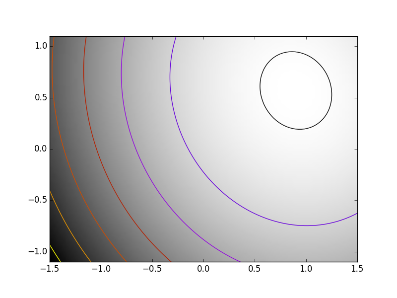
The challenge here is that Hessian of the problem is a very ill-conditioned matrix. This can easily be seen, as the Hessian of the first term in simply 2*np.dot(K.T, K). Thus the conditioning of the problem can be judged from looking at the conditioning of K.

スクリプトの出力:

  Powell: time 26.05s
       BFGS: time 22.02s, x error 2.66, f error 266.22
     L-BFGS: time 1.72s, x error 0.00, f error -0.00
  BFGS w f': time 3.41s, x error 2.66, f error 266.22
L-BFGS w f': time 0.15s, x error 0.00, f error -0.00
     Newton: time 0.34s, x error 2.66, f error 266.22

Python source code: plot_exercise_ill_conditioned.py

import time

import numpy as np
from scipy import optimize
import pylab as pl

np.random.seed(0)

K = np.random.normal(size=(100, 100))

def f(x):
    return np.sum((np.dot(K, x - 1))**2) + np.sum(x**2)**2


def f_prime(x):
    return 2*np.dot(np.dot(K.T, K), x - 1) + 4*np.sum(x**2)*x


def hessian(x):
    H = 2*np.dot(K.T, K) + 4*2*x*x[:, np.newaxis]
    return H + 4*np.eye(H.shape[0])*np.sum(x**2)


###############################################################################
# Some pretty plotting

pl.figure(1)
pl.clf()
Z = X, Y = np.mgrid[-1.5:1.5:100j, -1.1:1.1:100j]
# Complete in the additional dimensions with zeros
Z = np.reshape(Z, (2, -1)).copy()
Z.resize((100, Z.shape[-1]))
Z = np.apply_along_axis(f, 0, Z)
Z = np.reshape(Z, X.shape)
pl.imshow(Z.T, cmap=pl.cm.gray_r, extent=[-1.5, 1.5, -1.1, 1.1],
          origin='lower')
pl.contour(X, Y, Z, cmap=pl.cm.gnuplot)

# A reference but slow solution:
t0 = time.time()
x_ref = optimize.fmin_powell(f, K[0], xtol=1e-10, ftol=1e-6, disp=0)
print '     Powell: time %.2fs' % (time.time() - t0)
f_ref = f(x_ref)

# Compare different approaches
t0 = time.time()
x_bfgs = optimize.fmin_bfgs(f, K[0], disp=0)[0]
print '       BFGS: time %.2fs, x error %.2f, f error %.2f' % (time.time() - t0,
    np.sqrt(np.sum((x_bfgs - x_ref)**2)), f(x_bfgs) - f_ref)

t0 = time.time()
x_l_bfgs = optimize.fmin_l_bfgs_b(f, K[0], approx_grad=1, disp=0)[0]
print '     L-BFGS: time %.2fs, x error %.2f, f error %.2f' % (time.time() - t0,
    np.sqrt(np.sum((x_l_bfgs - x_ref)**2)), f(x_l_bfgs) - f_ref)


t0 = time.time()
x_bfgs = optimize.fmin_bfgs(f, K[0], f_prime, disp=0)[0]
print "  BFGS w f': time %.2fs, x error %.2f, f error %.2f" % (
    time.time() - t0, np.sqrt(np.sum((x_bfgs - x_ref)**2)),
    f(x_bfgs) - f_ref)

t0 = time.time()
x_l_bfgs = optimize.fmin_l_bfgs_b(f, K[0], f_prime, disp=0)[0]
print "L-BFGS w f': time %.2fs, x error %.2f, f error %.2f" % (
    time.time() - t0, np.sqrt(np.sum((x_l_bfgs - x_ref)**2)),
    f(x_l_bfgs) - f_ref)

t0 = time.time()
x_newton = optimize.fmin_ncg(f, K[0], f_prime, fhess=hessian, disp=0)[0]
print "     Newton: time %.2fs, x error %.2f, f error %.2f" % (
    time.time() - t0, np.sqrt(np.sum((x_newton - x_ref)**2)),
    f(x_newton) - f_ref)

pl.show()

Total running time of the example: 63.78 seconds ( 1 minutes 3.78 seconds)